DNA Metabarcoding

This repository contains the materials for the Metabarcoding day of the course “GENOMIC METHODS IN EVOLUTIONARY BIOLOGY AND ECOLOGY”. It deals with the methods to barcode diversity using amplicon sequencing (metabarcoding) with the help of a case study.

Github URL: https://github.com/claudioametrano/metab_db.git

Software required (on remote server)

• QIIME2

• Fastp

• FastQC

• MultiQC

Software required (locally)

• a fasta file reader (MEGA, Aliview, Jalview, Bioedit …)

• Terminal (Linux and Mac) or Mobaxterm (Win) toconnect to the remote server via SSH and a client (e.g. Mobaxterm, Filezilla) for easier file transfer

Introduction

Nucleotide reference databases for metabarcoding and diversity assessment (an example of secondary database)

Since the introduction of the high throughput sequencing technologies in the mid-2000s (Illumina, formerly Solexa; Roche 454; ABI SOLiD), metabarcoding has unlocked the unprecedented possibility of barcoding diversity, by enabling the simultaneous recovery of thousands of taxonomic signatures in a single run. Yet, the power of this approach depends on comprehensive, accurately curated reference databases for the most widely used “universal” barcodes (e.g., COI, 16S, ITS), without which the sequence output cannot be reliably linked to taxa identities. Most of them are a reduced, curated (and often clustered) version of NCBI GenBank (or similar databases).

Why reference databases are crucial:

• Taxonomic anchor: Metabarcoding reads are just strings of bases until they can be matched to a reference sequence; curated databases turn anonymous fragments, grouped into OUTs (Operational Taxonomic Units), into named taxa, giving ecological meaning to the data.

• Accuracy: Curated reference libraries increase the accuracy of taxonomic assignment of metabarcoding data diminishing, mis-labelled, chimeric and artifact sequences. This is critical for decision making based on biodiversity trend, or control of biological matrices (e.g. yes, multi-flower honey, but from what flowers?! plosone; appl. pl. sci.).

• Breadth of coverage: Comprehensive, standardized region-specific reference set minimizes the microbial “dark-matter” problem (Nature), making community profiles more complete, and analyses more reproducible and comparable across studies.

• Continuous update: Because taxonomy and sequence diversity keep changing and growing, regularly updated databases provide a mechanism to incorporate new barcodes and revised names, ensuring metabarcoding results stay interpretable over time.

Common Reference Databases for Metabarcoding

Marker	Taxa Focus	Database	Link / Notes
COI (rbcL, matk, ITS, 18S)	Animals (plants, fungi)	BOLD: Barcode Of Life Database	bold
COI (additional mito markers)	Animals (and other eukaryotes)	MIDORI	midori2
ITS	Fungi (plants, other eukaryotes)	UNITE	unite
ITS	plants	PLANiTS	https://academic.oup.com/database/article/doi/10.1093/database/baz155/5722079
18S rRNA, full rDNA	Eukaryotes	PR2	pr2
16S/18S, 23S/28S rRNA	Bacteria, Archaea and Eukarya	SILVA	silva
16S rRNA	Bacteria, Archaea	Greengenes	https://www.nature.com/articles/s41587-023-01845-1

These databases have usually a very simple structure, they are made by one or two files, containing:

• Reference sequences (usually in .fasta format)

• A taxonomy file with the taxonomy associated to each of the representative sequence

Tools and pipelines commonly used in metabarcoding

After about two decades of metabarcoding there are plenty of tools and pipelines which were developed to analyze metabarcoding data, many of them composed by the same fundamental steps, also often sharing methods and piece of software (e.g. QIIME using DADA2 denoising algorithm)

Pipeline / Platform	Core language & interface	Main approach (ASV vs OTU, multi-marker, etc.)	Reference
QIIME 2	Python + plugin framework (CLI, GUI, Galaxy)	Flexible; ASV (DADA2/Deblur) or OTU; integrates phylogenetics & statistics	qiime2
DADA2	R package	Denoising → exact Amplicon Sequence Variants (ASVs)	dada2
mothur	C++ binary with command shell	OTU clustering (97 %), plus chimera checking	https://mothur.org
OBITools	Python scripts	Read filtering, taxonomic assignment, ecology metrics	obitools
Anacapa Toolkit	Conda/R + Snakemake	Multi-locus (COI, 12S, 18S) with custom reference building	GitHub
MetaWorks	Snakemake workflow (Python/R)	Multi-locus (ITS, COI) with VSEARCH + tax-assign	GitHub
mBRAVE	Web cloud platform	OTU/ASV assignment against curated BOLD	mbrave.net

A typical metabarcoding experiment workflow

modif. from Pawlowsky et al. 2018

Phase 1: Experimental design

• Question to answer using amplicon sequencing data

• Actual design: How many samples/replicates? How many markers/which organims target? How many libraries? What expected sequencing depth? How large is the budget?

• Metadata: by direct measurments? from public databases?

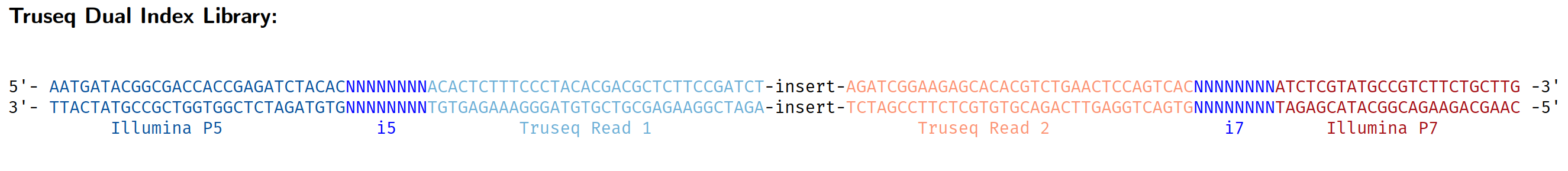
Phase 2: Library preparation

from Illumina

Phase 3: Data analysis

This is an overview from QIIME2 website, but many of these steps are similar no matter what pipeline you select

NOTE

AVS vs OTU: OTU (Operational Taxonomic Unit) A pragmatic “species-proxy” label assigned to a cluster of metabarcoding reads that are ≥ x % similar (most often 97-99 %). ASV (Amplicon Sequence Variant) An “exact”, denoised biological sequence present in the sample. Single-nucleotide resolution rather than an arbitrary similarity bin.

NOTE bis

After the overview of the method, do you think metabarcoding is a quantitative method? Does it model accurately the abundance of the original meta-genomic DNA extracted from environmental matrices (e.g. soil, water, …)

BEFORE WE START

Login to your account on the HPC remote server and start an interactive session

$ ssh username@l2.gsc1.uni-graz.at

$ srun --mem=16G --ntasks=1 --cpus-per-task=8 --time=10:00:00 --pty bash

Download this repository:

$ git clone https://github.com/claudioametrano/metab_db.git

Create the results folder

$ cd metab_db  
$ mkdir results

Case study: welcome to the Trieste coast, a “toy” 16S dataset

We are not going to produce our own data, we will instead use a toy version of an actual experiment. The data were subsampled (1%) from the Illumina sequencing of a 16S rDNA library, produced to assess the prokaryotic diversity in a coastal environment, in different experimental conditions and sites. biochar paper here

from Fukuda et al. 2016

1. Required data:

• Sequences (fastq) -> data/16S_biochar_run2_1perc/

• Metadata -> ./data/metadada.csv let’s take a look at them to understad the experimental design

• Reference database -> SILVA

If you are not already in the repository main directory go there:

$ cd metab_db

Caution

All the command from now ahead are lauched with the relative path starting from the current directory, which is the main folder of this repository

• Check the sequence data file without decompressing them, which kind of data is this?

• Count the number of sequences per file

• How long are the reads? (hint: use zless or zcat, zgrep and awk with length)

2. Reads QC and trimming

2.1 Raw reads quality control

Command line is great (he said), quick and versatile, but user friendly, interactive .html quality report are generated by software such as FastQC and MultiQC

We will run them via existing containers: FastQC to benchmark each sample

$ mkdir ./results/fastqc_raw_out

$ singularity pull https://depot.galaxyproject.org/singularity/fastqc:0.12.1--hdfd78af_0

$ singularity shell fastqc:0.12.1--hdfd78af_0
 
$ fastqc data/16S_biochar_run2_1perc/*.gz -o results/fastqc_raw_out --threads 4 --nogroup

$ exit

The same command can be launched in the container without necessary remaining in an interactive session:

$ singularity exec fastqc\:0.12.1--hdfd78af_0 fastqc data/16S_biochar_run2_1perc/*.gz -o results/fastqc_raw_out --threads 8 --nogroup

MultiQC aggregates results to highlight possible outliers

$ mkdir ./results/multiqc_raw_out

$ singularity pull https://depot.galaxyproject.org/singularity/multiqc:1.26--pyhdfd78af_0

$ singularity exec multiqc\:1.26--pyhdfd78af_0 multiqc results/fastqc_raw_out/ -o results/multiqc_raw_out

TASK2

Now check the .html output of R1 and R2 fastq file from some of the samples (download it from server by Filezilla or any other client) and the aggregated report of MultuQC and try to answer the following questions:

• 1. Which of the warnings thrown by fasQC are of actual concern, and which are not? Why?

• 2. Do you notice any difference in term of quality between corresponding R1 and R2 files?

• 3. Does any sample show peculiar characteristics in term of quality, nucleotide composition, etc?

• 4. If any, what are the over-represented sequences? Are they of concern for subsequent analyses?

• 5. Does your sequence contains residual Illumina adapters/sequencing primers and marker’s primers?

• 6. Could you explain why polyG sequences are common? Do they have biological meaning? (hint: look at bottom-right corner of the Library Preparation figure)

Optional: explore low CG content reads peak (see fastQC and MultiQC report) present in some samples

$ mkdir results/GC_extreme
# Copy the script to select reads by CG content and one relevant fastq into the folder
$ cp data/16S_biochar_run2_1perc/*S41*R2* results/GC_extreme/
$ gunzip results/GC_extreme/Bch-16S-V3V4-041-2_S41_L002_R2_001.fastq_1perc.fastq.gz
$ cp solutions/select_fastq_reads_by_GC_cont.py results/GC_extreme/
# The script we are goinmg to use requires BioPython
$ singularity pull https://depot.galaxyproject.org/singularity/biopython:1.79
$ singularity shell biopython\:1.79
$ cd results/GC_extreme/
# Run the script that selects reads by GC content, and output them in fasta
$ python select_fastq_reads_by_GC_cont.py 
# select file name and GC content range and BLAST some of the results
$ exit

taken from this informative website

TASK3

FastQC do not search for your custom primer (well, not by default) so now it is your turn to do so: Primer for 16S rRNA (V3-V4 region)

Forward: Pro341F (5’-CCTACGGGNBGCASCAG-3’)

Reverse: Pro805R (5’-GACTACNVGGGTATCTAATCC-3’)]

Do you notice anything unusual? IUPAC nucleotide code

Questions:

• Do all sequence have primers? Where in the sequence?

• Is there any sequence that do not match your search? if so, why? (hint: use zgrep with regular expression (-E) and the regex e.g. “[A | T]” when more than one character is possible, see grep –help. Note that “|” has a different meaning in regex than it has as a pipe, here it means OR)

2.2 Quality trimming and adapter removal

Many software are available (fastp, Trimmomatic, cutadapt etc.) with various option and approaches to trimming, removing adapters and/or primers, even though these reads are of really have quality and denoising algoritm work usually well with raw reads, there is a little room for improvement (let’s check after the trimming if it is worth it)

Fastp is one of the most versatile tool to pre-process short reads, unfortunately id does not seem to support degenerate primers

$ mkdir ./results/trimmed_fastq
$ mkdir ./results/report_fastp

$ singularity pull https://depot.galaxyproject.org/singularity/fastp:0.24.0--heae3180_1

$ singularity shell  fastp:0.24.0--heae3180_1

The following is a Bash script that runs fastp for each of the paired fastq files… it will take a while even with this toy dataset, while it runs let’s take a look at the script here below

IN_DIR="data/16S_biochar_run2_1perc"
OUT_DIR="results/trimmed_fastq"
OUT_REPORT="/results/report_fastp"

for r1 in "$IN_DIR"/*_R1_001.fastq_1perc.fastq.gz; do
    # strip the long suffix first
    sample_path=${r1%_R1_001.fastq_1perc.fastq.gz}
    # keep only the sample name
    sample=$(basename "$sample_path")

    r2="$IN_DIR/${sample}_R2_001.fastq_1perc.fastq.gz"

    echo "Trimming sample: $sample"

    fastp \
        -i  "$r1" \
        -I  "$r2" \
        -o  "${OUT_DIR}/${sample}_R1.trimmed.fastq.gz" \
        -O  "${OUT_DIR}/${sample}_R2.trimmed.fastq.gz" \
        --detect_adapter_for_pe \
        --trim_poly_x \
        --trim_tail1 0 \
        --trim_tail2 0 \
        --trim_front1 17 \
        --trim_front2 21 \
        --cut_front --cut_tail \
        --cut_window_size 4 \
        --cut_mean_quality 30 \
        --qualified_quality_phred 30 \
        --length_required 200 \
        --thread 8 \
        --html "${OUT_REPORT}/${sample}.html" \
        --json "${OUT_REPORT}/${sample}.json" \
    echo "Done with $sample"
done

$ exit

NOTE

This could have been carried out in a more elegant way putting the script in a file and launcing in a singularity exec command, but we took the chance to take a look at the script!

TASK 4

Search in the fastp manual what are the options -trim_front1 17 -trim_front2 21 and try to guess why those numbers were picked? Can you also propose a more refined solution to solve the same issue?

2.3 Trimmed reads quality

Run again fastQC and MultiQC (in a different output folder!!) and check what happened.

$ mkdir ./results/fastqc_trimmed_out

$ singularity exec  fastqc\:0.12.1--hdfd78af_0 fastqc results/trimmed_fastq/*.gz -o results/fastqc_trimmed_out --threads 8 --nogroup

$ mkdir ./results/multiqc_trimmed_out

$ singularity exec  multiqc\:1.26--pyhdfd78af_0 multiqc results/fastqc_trimmed_out/ -o results/multiqc_trimmed_out

The QIIME environment

Recently converted to a microbiome multi-omics data science platform, it started as a user-friendly command line software (written in Python) to analyze NGS amplicon sequencing data.

Obtain and test qiime container

$ singularity pull docker://quay.io/qiime2/amplicon:2024.10

$ singularity exec --home "$(pwd)":/home/qiime2 amplicon_2024.10.sif qiime --help

qiime tries to create a small cache under /home/qiime2/ so we need to mount also the qiime home folder.

NOTE

you can choose to run the qiime command using its containerized version either interactively, using singularity shell or not, using singularity exec. > If you decide to run it interactively you can activate tab-completion. See the box below:

$ singularity shell --home "$(pwd)":/home/qiime2 amplicon_2024.10.sif

# to activate tab-completion
$ source tab-qiime

$ exit

Import data into QIIME

$ mkdir ./results/qiime_artifacts/

$ singularity exec --home "$(pwd)":/home/qiime2 amplicon_2024.10.sif qiime tools import   --type 'SampleData[PairedEndSequencesWithQuality]'   --input-path results/trimmed_fastq/ --input-format CasavaOneEightSingleLanePerSampleDirFmt --output-path results/qiime_artifacts/16S_biochar.qza

Something went wrong importing, can you tell why and find a solution to it?

$ singularity pull https://depot.galaxyproject.org/singularity/rename:1.601--hdfd78af_1

$ singularity exec rename\:1.601--hdfd78af_1 rename 's/.trimmed.fastq.gz/_001.fastq.gz/' results/trimmed_fastq/*.gz

Now go back to QIIME container and re-try importing your fastq files, it should work…

GOOD, CONGRATS! … you imported your first dataset into QIIME

3. Denoising and AVS table

This step is quite slow even with only 10000 read as training set for DADA2 (~ 10 mins with 8 threads of AMD EPYC 9825):hourglass: … :coffe: break?

$ singularity exec --home "$(pwd)":/home/qiime2 amplicon_2024.10.sif qiime dada2 denoise-paired \
  --p-n-threads 8\
  --p-trunc-len-f 0 \
  --p-trunc-len-r 0 \
  --i-demultiplexed-seqs results/qiime_artifacts/16S_biochar.qza \
  --o-representative-sequences results/qiime_artifacts/rep-seqs.qza \
  --o-table results/qiime_artifacts/asv-table.qza \
  --o-denoising-stats results/qiime_artifacts/stats.qza \
  --p-min-overlap 12 \
  --p-n-reads-learn 10000

This command will produce two outputs which are the fundamental pieces of any matabarcoding analysis:

• an ASV/OTU table

• a fasta containing the representative sequence of each of the detected ASV/OTU A report showing the step to get the ASV with DADA (Divisive Amplicon Denoising Algorithm) denoising method.

TASK 5

Find your way of visualizing the stat.qza content without using Qiime embedded visualizations hint: Qiime .qza files are simply (zip) compressed archives What do you notice being the step mostly influencing the number of surviving sequences? Can you guess why?

Visualization of ASV table and representative sequences

Qiime is a user friendly platform which integrates visualization and diversity/ecology analyses, let’s take a look at them

$ singularity exec --home "$(pwd)":/home/qiime2 amplicon_2024.10.sif qiime feature-table summarize \
  --i-table results/qiime_artifacts/asv-table.qza \
  --o-visualization results/qiime_artifacts/asv-table.qzv \
  --m-sample-metadata-file data/metadata.csv

$ singularity exec --home "$(pwd)":/home/qiime2 amplicon_2024.10.sif qiime feature-table tabulate-seqs \
  --i-data results/qiime_artifacts/rep-seqs.qza \
  --o-visualization results/qiime_artifacts/rep-seqs.qzv

Now download the .qzv files and drag & drop in the window at QIIME view. This way you can visualize the ASVs (called feature, in QIIME) and their sequence, and a simple statistic of the ASV dstribution in samples.

To visualize the actual ASV table we need to introduce another common file format in bioinformatics: BIOM format (BIological Observation Matrix)

# extract using 7zip
$ 7z x ./results/qiime_artifacts/asv-table.qza -o./results/qiime_artifacts/

# or using unzip
$ unzip ./results/qiime_artifacts/asv-table.qza -d ./results/qiime_artifacts/

# name_of_the_folder according to the actual name
$ singularity exec  --home "$(pwd)":/home/qiime2 amplicon_2024.10.sif biom convert -i ./results/qiime_artifacts/name_of_the_folder/data/feature-table.biom -o ./results/asv-table.tsv --to-tsv

$ less -S results/asv-table.tsv

Observing the table and the frequencies of features (ASVs) it is clear that metabarcoding data (especially when relying on ASVs as unit) are characterized by sparsity: the scenario where a large percentage of data within a dataset is missing or is set to zero. Possible strategy to limit this data issue:

• Cluster ASVs into OTUs

• Remove ASV with extremely low abundance and sample frequency across samples.

Remove extremely rare ASVs

…which are more prone to be sequencing errors. It also diminishes the final matrix sparsity

$ singularity exec  --home "$(pwd)":/home/qiime2 amplicon_2024.10.sif qiime feature-table filter-features \
--i-table results/qiime_artifacts/asv-table.qza \
--p-min-frequency 10 \
--p-min-samples   2 \
--o-filtered-table results/qiime_artifacts/asv-table_norare.qza

4. Alpha rarefaction curves

Rarefaction is a method used both to normalize metabarcoding data, here is used as a preliminary assessment of sampling effort, to see if it was enough to describe the target microbial community diversity

$ singularity exec --home "$(pwd)":/home/qiime2 amplicon_2024.10.sif qiime diversity alpha-rarefaction \
--i-table ./results/qiime_artifacts/asv-table_norare.qza \
--p-max-depth xxx \
--p-steps xxx \
--m-metadata-file ./data/metadata.csv \
--o-visualization ./results/qiime_artifacts/alpha-rarefaction.qzv	

TASK6

Select suitable resampling depth and step values for the rarefaction analysis (hint: search in --help of the diversity alpha-rarefaction command)

Visualize the results in QIIME view

5. Taxonomic assignment

Finally we are getting to the part where the ecological meaning of our data can be investigated, first thing first, we would like to know who we are dealing with, to do so we need to assign taxonomy to our ASVs using a reference database

Obtain the reference database

Let’s download the latest version of SILVA 99% similarity clustered version, pre-formatted for QIIME, if you are curious take a look inside (they are just regular zipfiles) to see how the taxonomy format looks like

$ cd results/qiime_artifacts

$ wget https://data.qiime2.org/2023.2/common/silva-138-99-seqs.qza
$ wget https://data.qiime2.org/2023.2/common/silva-138-99-tax.qza
$ cd ../..

Resize the database to V3-V4 region only, based on primer system used

We are going to use our database with a method base on k-mer composition, therefore is beneficial to retain only the 16S region (V3-V4) amplified by our primers. If using an alignment method, shorter reference database will improve speed and resource use. This will take quite long (~30 mins on 70 thread of AMD EPYC 9825 CPU) :hourglass:

$ singularity exec --home "$(pwd)":/home/qiime2 amplicon_2024.10.sif   qiime feature-classifier extract-reads \
--i-sequences results/qiime_artifacts/silva-138-99-seqs.qza \
--p-f-primer CCTACGGGNBGCASCAG \
--p-r-primer GACTACNVGGGTATCTAATCC \
--p-read-orientation both \
--p-identity 0.80 \
--p-n-jobs 8 \
--o-reads results/qiime_artifacts/silva-138-99-v3v4-seqs.qza \
--verbose

Train a classifier

Since reference sequences and the relative taxonomy are already imported in QIIME format we can train an object whose purpose is to assign taxonomy to our ASVs: Naive Bayes classifier It is a supervised machine learning model that uses k-mer composition or reference database (and reads) to assign a taxonomy

$ singularity exec  --home "$(pwd)":/home/qiime2 amplicon_2024.10.sif qiime feature-classifier fit-classifier-naive-bayes \
  --i-reference-reads results/silva-138-99-v3v4-seqs.qza \
  --i-reference-taxonomy results/silva-138-99-tax.qza \
  --o-classifier results/qiime_artifacts/classifier_silva138_99-v3v4.qza

as the training can run for very long ( ~1h on one thread of AMD EPYC 9825 CPU, not parallelized) :hourglass: and can require a lot of RAM (up to ~24 Gb for this 16S v3-v4 classifier) , abort it with ctrl+C, we will use an already trained classifier: classifier_silva-v3v4-138_99.qza

Classify the representative sequences associated to each ASV

Now that we have the classifier we can use it to classify our sequences… or at least try (~15 min on 20 thread of AMD EPYC 9825 CPU) :hourglass:

$ singularity exec --home "$(pwd)":/home/qiime2 amplicon_2024.10.sif qiime feature-classifier classify-sklearn \
  --p-n-jobs 8 \
  --i-classifier results/qiime_artifacts/classifier_silva138_99-v3v4.qza \
  --i-reads results/qiime_artifacts/rep-seqs.qza \
  --o-classification results/qiime_artifacts/taxonomy.qza \
  --p-reads-per-batch 100

If we fail due RAM constraint to train a classifier, we may try another taxonomic assignment approach, for example one based on the alignment of AVS sequences to the database, such as the global alignment with VSEARCH

$ singularity exec --home "$(pwd)":/home/qiime2 amplicon_2024.10.sif qiime feature-classifier classify-consensus-vsearch \
  --i-query            rep-seqs.qza \
  --i-reference-reads  silva-138-99-seqs.qza \
  --i-reference-taxonomy silva-138-99-tax.qza \
  --p-perc-identity    0.97 \
  --p-query-cov        0.80 \
  --p-min-consensus    0.80 \
  --p-maxaccepts       10 \
  --p-strand           both \
  --p-top-hits-only    \
  --p-threads          8 \
  --o-classification   taxonomy.qza \
  --o-search-results   vsearch_hits.qza \
  --verbose

This is not as memory intensive as training a classifier but can run for long (depending on computational resources). In alternative, we can retrieve the already classified ASV from a previous run: taxonomy.qza

Plot taxonomic composition of samples

$ singularity exec --home "$(pwd)":/home/qiime2 amplicon_2024.10.sif qiime taxa barplot \
  --i-table results/qiime_artifacts/asv-table_norare.qza \
  --i-taxonomy results/qiime_artifacts/taxonomy.qza \
  --m-metadata-file data/metadata.csv \
  --o-visualization results/qiime_artifacts/taxa-bar-plots.qzv

TASK 7

Explore the interactive bar-plots, is it anything you would exclude for subsequent diversity analyses of the prokaryotic community?

Filter the ASVs table using assigned taxonomy

$ singularity exec --home "$(pwd)":/home/qiime2 amplicon_2024.10.sif qiime taxa filter-table \
--i-table results/qiime_artifacts/asv-table_norare.qza \
--i-taxonomy results/qiime_artifacts/taxonomy.qza \
--p-exclude Mitochondria,Chloroplast \
--o-filtered-table results/qiime_artifacts/asv-table_norare_mito_chl_taxfiltered.qza \
--verbose

6 Diversity analyses: alpha and beta diversity (Whittaker, 1972)

Alpha diversity: the within-community component of biodiversity, the effective number of distinct taxa in a single, spatially homogeneous sample.

Reducing each sample to a diversity index, a single numerical value, is one of the most common operation performed on the ASV/OTU table, it comes at the cost of loosing most of the information stored in the AVS/OTU table, but can highlight relevant differences among the investigated communities.

Indices automatically calculated by QIIME pipeline

• Observed Features

• Shannon’s diversity index

• Faith’s Phylogenetic Diversity (a qualitative measure of community richness that incorporates phylogenetic relationships between the features)

• Pielou’s Evenness

Beta diversity: a measure of variation in species composition between ecological communities or across spatial or environmental gradients. It quantifies the degree to which communities differ from one another in their species composition.

ASV table -> Distance/similarity index among samples -> distance/similarity matrix -> Ordination (PCoA, mMDS, …) and statistics to test the differences among (microbial) communities in different conditions (according to metadata) such as PERMANOVA

As some alpha diversity metrics also include phylogenetic distance in their formula, we are now inferring a (not particularly accurate… why?) phylogenetic tree based on the representative sequences of our ASVs

$ singularity exec --home "$(pwd)":/home/qiime2 amplicon_2024.10.sif qiime phylogeny align-to-tree-mafft-fasttree \
  --i-sequences results/qiime_artifacts/rep-seqs.qza \
  --o-alignment results/qiime_artifacts/aligned-rep-seqs.qza \
  --o-masked-alignment results/qiime_artifacts/masked-aligned-rep-seqs.qza \
  --o-tree results/qiime_artifacts/unrooted-tree.qza \
  --o-rooted-tree results/qiime_artifacts/rooted-tree.qza \
  --p-n-threads 8

Alpha and beta diversity calculation

$ singularity exec  --home "$(pwd)":/home/qiime2 amplicon_2024.10.sif qiime diversity core-metrics-phylogenetic \
  --i-phylogeny results/qiime_artifacts/rooted-tree.qza \
  --i-table results/qiime_artifacts/asv-table_norare_mito_chl_taxfiltered.qza \
  --p-sampling-depth xxx \
  --m-metadata-file data/metadata.csv \
  --output-dir results/qiime_artifacts/diversity-core-metrics-phylogenetic

Pick a suitable value for --p-sampling-depth : what method are you applying to normalize samples? What is the best trade off between sampling depth and samples lost?

TASK 8

Explore the ordinations produced (e.g. bray_curtis_emperor.qzv ). Can you identify a metadata (e.g. Time, Location, Substrate, …) that seems to be informative according to the ordination plot?

Hypotheses testing with alpha diversity

For example using the Observed features (the raw number of ASV, without applying diversity indices)

$ singularity exec --home "$(pwd)":/home/qiime2 amplicon_2024.10.sif qiime diversity alpha-group-significance \
  --i-alpha-diversity results/qiime_artifacts/diversity-core-metrics-phylogenetic/observed_features_vector.qza \
  --m-metadata-file data/metadata.csv \
  --o-visualization results/qiime_artifacts/diversity-core-metrics-phylogenetic/observed_features-significance.qzv

TASK 9

Try modifying the previous command in order to statistically test hypotheses using other diversity indices? Is any significant difference highlighted? Can you draw any conclusion?

…and beta diversity using PERMANOVA (Anderson, 2001)

The following commands will test whether distances between samples within a group, are more similar to each other then they are to samples from the other groups. If you call this command with the --p-pairwise parameter, it will also perform pairwise tests that will allow you to determine which specific pairs of groups differ from one another, if any. In a nutshell: PERMANOVA compares between-group variation to within-group variation. Significance is assessed by repeatedly permuting group labels and recalculating the pseudo-F statistic. It answers to the question: “Are samples from the same metadata group more similar to each other than expected by chance?”

$ singularity exec  --home "$(pwd)":/home/qiime2 amplicon_2024.10.sif \
qiime diversity beta-group-significance \
  --i-distance-matrix results/qiime_artifacts/diversity-core-metrics-phylogenetic/bray_curtis_distance_matrix.qza \
  --m-metadata-file data/metadata.csv \
  --m-metadata-column Substrate \
  --o-visualization results/qiime_artifacts/diversity-core-metrics-phylogenetic/bray_curtis-substrate-significance.qzv \
  --p-pairwise

Test also different grouping to highlight significant differences, what would you use given the previous results?

FINAL TASK

BUILD A REPORT CONTAINING EVERY STEP YOU TOOK, REPORTING THE COMMANDS USED AND THEIR OUTPUT (meaningful examples or summary tables are enough if the output is large!). IT CAN BE DELIVERED IN .docx, .pdf, OR MARKDOWN TEXT FILE.

1. Pick a metabarcoding study from literature, with the following characteristics:

• A reasonable amount of samples (metabarcoding surveys can be huge, even though per single sample data are usually quite manageable -> short reads amplicon sequencing).

• Based on one barcode (if multiple barcodes libraries are used in the manuscript, you can select one, and only work on a subset of samples)

• Clearly explained and reproducible methods

• Raw sequences available (e.g. at NCBI SRA)

• Available metadata files

• It can be from whatever matrix, you have maximum freedom to select something which intrigues you. Some examples: Human gut/oral/skin/… microbiota, eDNA from water, air (yes, aerobiology does exists), soil, aerosol, plant, fungal, animal microbiota, honey, etc.

2. Identifiy the aim of the study.

3. Reproduce the main basic steps of a metabarcoding analysis following the main step we performed (from raw sequences, to diversity analyses and hypotheses testing using metadata).

4. Critically Compare the method and the results you obtained with the methods and results from the paper you selected (they do not need to be exactly the same, as you are restricted to QIIME):

• Did you use the same tool/pipeline the authors used to perform the analyses? List methods and highlight differencies explaining your chioice (e.g for sequence data filtering/trimming, OTU clustering or ASV, similarity thresholds applied, data normalization method, alpha and beta diversity methods applied, statistics).

• Could you get to their same conclusions? Describe the results, and how data were suitable to verify the hypotheses of the study.

• Did the change of method noticeably affect the results? If that happened what were the main differences?